Food Image Recognition for Recipe Retrieval
Muriz Serifovic
2018-09-09
Originally published in Towards Data Science ↗
A convolutional network over 800,000 food photographs and 300,000 recipes from chefkoch.de
Introduction
 This article looks at training a deep convolutional neural network capable of classifying images into food categories and outputting a matching recipe. The chosen target domain is hard for two reasons. First, progress on the classification or object recognition of individual ingredients of cooking dishes is sparse, because virtually no public processed datasets exist for it. Second, cooking dishes have an intrinsically high inter-class similarity, which makes deducing a dish's category a difficult problem even for the most sophisticated systems. To tackle these challenges we scrape a novel dataset of more than 800,000 food images and more than 300,000 recipes from one of Europe's most popular cooking platforms, chefkoch.de, and empirically compare contemporary machine-learning models (convolutional neural networks) against more traditional methods (nearest-neighbour search).
Preface
Hardly any other area influences human well-being to the same extent as nutrition. Each day an innumerable amount of food pictures is posted by users on social networks; from the first homemade cake to the top Michelin dish, people are happy to share their joy with the world when a dish succeeds. No matter how different one person is from another, good food is appreciated by just about everyone.
Advances in the classification of individual cooking ingredients are sparse, again because almost no public edited records are available. This work addresses the automated recognition of a photographed cooking dish and the subsequent output of the appropriate recipe. What sets it apart from earlier supervised classification problems is the large overlap between food dishes — a high inter-class similarity — because dishes of different categories can look very similar in terms of image information alone (see Figure 1).
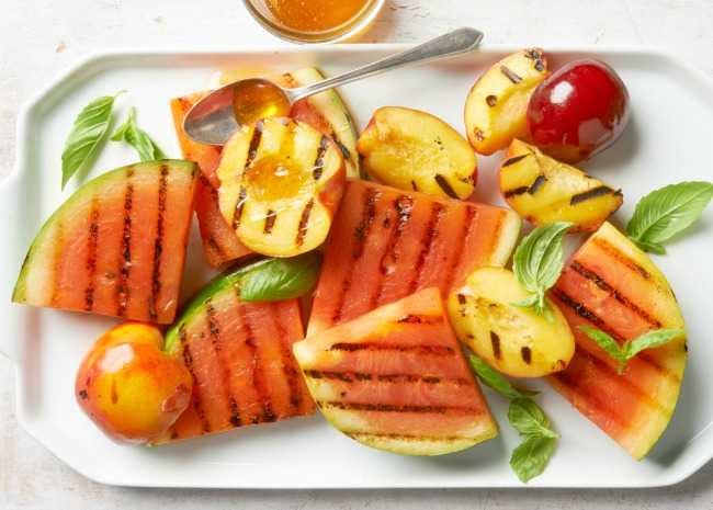
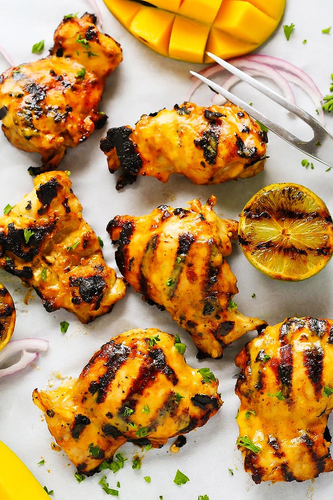
The tutorial is subdivided into smaller parts in line with the motto divide and conquer. To the current state of the art, this scrapes and analyses the largest German-language dataset of more than 300,000 recipes. We postulate that machine learning may overcome the hurdles of more traditional query methods: we combine object recognition (dish recognition) using convolutional neural networks — CNN for short — with a search for the nearest neighbours (next-neighbour classification) over a record of more than 800,000 images. This combination may help find the recipe more reliably and steer classification in more fruitful directions, because the top-k categories of the CNN are compared with the next-neighbour category by ranked correlation. Rank-correlation approaches such as Kendall Tau essentially measure the probability of two items appearing in the same order in the two ranked lists. Kendall Tau is computed as $$ \tau = \frac{C - D}{\tfrac{1}{2}\,N\,(N-1)} $$ where
- $N$ = total number of pairs
- $C$ = number of concordant pairs
- $D$ = number of discordant pairs
Methodology
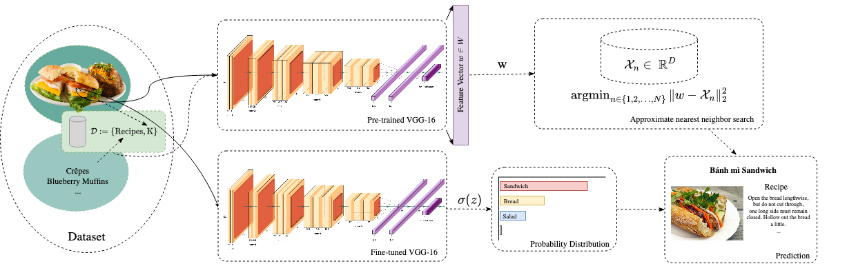
The pipeline is described by the following steps:
- Each recipe R is composed of K pictures. For each of these images a feature vector w ∈ W is extracted from a pre-trained convolutional neural network — one pre-trained on millions of images across the 1,000 categories of the ILSVRC 2014 image-recognition competition. Loosely speaking, the feature vectors form an internal representation of the image in the last fully connected layer, just before the 1,000-category Softmax layer.
- These feature vectors W are then dimensionally reduced by PCA (Principal Component Analysis) from an N × 4096 matrix to an N × 512 matrix. From the result one chooses the top-k images with the smallest Euclidean distance to the input image. Because computing a pairwise distance metric is computationally intensive and does not scale well, we turn to the approximate variant, ANN (approximate nearest neighbour).
- Furthermore, a CNN is trained with categories C on pictures of the R recipes. The number C is determined dynamically using a popular topic-modeling technique called non-negative matrix factorization (NNMF) and semantic analysis of recipe names. As a result we obtain, for each image in a recipe r ∈ R, a probability distribution over the categories.
- The top-k categories from the CNN (step 2) are compared with the categories from the top-k optically similar images (step 1) via Kendall Tau correlation.
The general method is outlined in Figure 2:
The work is organized into the following parts, each with accompanying Jupyter notebooks on the GitHub page:
- Data preparation — clearing data; data augmentation.
- Data analysis and visualization; splitting the data into train, valid and test.
- Topic modeling — Latent Dirichlet Allocation (LDA); Non-negative Matrix Factorization.
- Feature extraction — k-nearest neighbours; t-SNE visualization.
- Transfer learning — training a pre-trained CNN (AlexNet, VGG, ResNet, GoogLeNet).
- Deploying with Flask.
Scraping and preparing the data
Before any of it can run, somebody has to go and fetch three hundred thousand recipes, which takes considerably longer than choosing between LDA and NMF.
To train a model at all, one needs a sufficient amount of data — and where the raw quantity falls short, data augmentation and the fine-tuning of pre-trained models provide a remedy. Only with enough data can the generalization of the training set be increased to a useful degree and a high accuracy reached on the test set. This first part deals with data acquisition, analysis and the visualization of features and their relationships.
Peter Norvig, Google's Director of Research, put it memorably in a 2011 interview: "We do not have better algorithms. We just have more data." Without exception, the quality and quantity of the dataset is not negligible. That is why Europe's biggest cooking platform was scraped: every recipe — finally 316,756 recipes as of December 2017 — was downloaded, together with a total of 879,620 images. It is important not to proceed too quickly when downloading, and to spare the servers excessive queries, since otherwise a ban of one's own IP address would make data collection more difficult.
More data leads to more dimensions, but more dimensions do not necessarily lead to a better model or a better representation. Deviating patterns in the dataset that disturb learning can be unintentionally amplified by more dimensions; generalization and learning are then impaired for the neural network, and the signal-to-noise ratio decreases.
When scraping a website it is important to respect the robots.txt file: some administrators do not want bot visits to specific directories. The directories chefkoch.de disallows are not ones we are interested in, so collection can continue — though measures such as randomized headers and sufficiently large pauses between requests are still recommended to avoid a ban. The first pass collects the recipe name, the average rating, the number of ratings, the difficulty level, the preparation time and the publication date; the second pass collects the ingredient list, the recipe text, all images, and the number of times the recipe has been printed. These features describe the dataset well and help build a strong understanding of it, which is important when choosing algorithms.
The starting point is the paginated recipe index, from which the total number of pages is read:
# Chefkoch.de website
CHEFKOCH_URL = 'http://www.chefkoch.de'
START_URL = 'http://www.chefkoch.de/rs/s'
CATEGORY = '/Rezepte.html'
category_url = START_URL + '0o3' + CATEGORY

def _get_html(url):
    page = ''
    while page == '':
        try:
            page = requests.get(url, headers=random_headers())
        except:
            print('Connection refused')
            time.sleep(10)
            continue
    return page.text

def _get_total_pages(html):
    soup = BeautifulSoup(html, 'lxml')
    total_pages = soup.find('div', class_='ck-pagination qa-pagination') \
                      .find('a', class_='qa-pagination-pagelink-last').text
    return int(total_pages)

html_text_total_pages = _get_html(category_url)
total_pages = _get_total_pages(html_text_total_pages)
print('Total pages: ', total_pages)
# Total pages: 10560
Recipe-level data such as the recipe name, rating and upload date are stored in a CSV file; if a recipe has an image, the thumbnail is placed in the search_thumbnails folder. We use multiprocessing to keep the download time short.For further information see Python's documentation.
def scrap_main(url):
    print('Current url: ', url)
    html = _get_html(url)
    _get_front_page(html)
    # sleep(randint(1, 2))

start_time = time()
with Pool(15) as p:
    p.map(scrap_main, url_list)
print("--- %s seconds ---" % (time() - start_time))
The given code has been shortened; for the full version see the corresponding Jupyter notebook. Next we scrape the ingredient list, the preparation steps, the tags and all images of each recipe:
def write_recipe_details(data):
    dpath = DATAST_FOLDER + DFILE_NAME
    with open(dpath, 'a', newline='') as f:
        writer = csv.writer(f)
        try:
            writer.writerow((data['link'],
                             data['ingredients'],
                             data['zubereitung'],
                             data['tags'],
                             data['gedruckt:'],
                             data['n_pics']
                             ))
        except:
            writer.writerow('')
If everything went smoothly with the download, our data looks like this:
- A total of 879,620 images (35 GB)
- 316,756 recipes
- Of which 189,969 contain one or more pictures
- Of which 107,052 recipes contain more than 2 images
- 126,787 contain no picture
- Of which 189,969 contain one or more pictures
Data analysis and visualization
Thirty-five gigabytes of other people’s dinners is impossible to hold in your head, and the first question is what is actually in it.
Statistics
To get a first impression we usually plot a heatmap, which gives early insight into which features might be interesting.
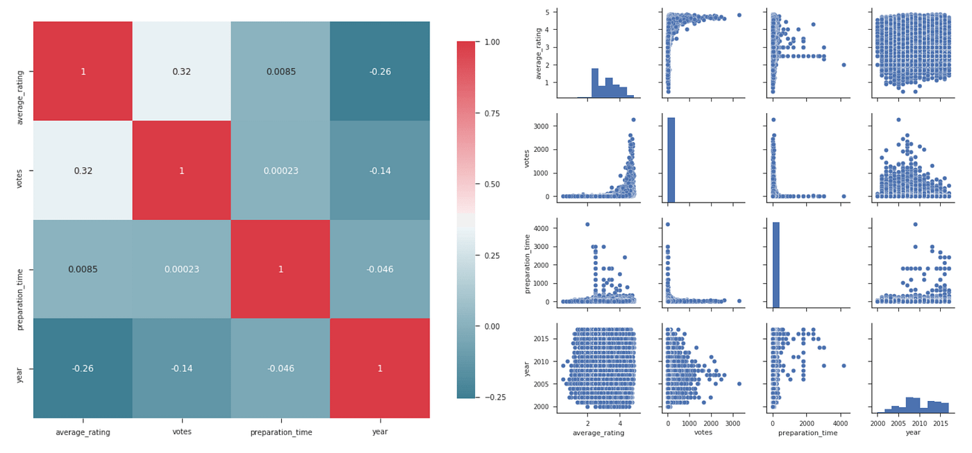
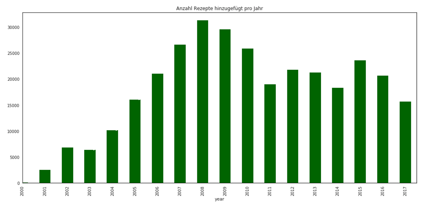
The highest correlation is between votes and average_rating. The pair plot makes it stand out that the higher the number of ratings, the better the rating of the recipe. The comparison between preparation time and number of ratings is also interesting: most reviews concern recipes with short preparation times, so it seems the ChefKoch community prefers easy recipes. Another idea is to compare the number of newly uploaded recipes per year.
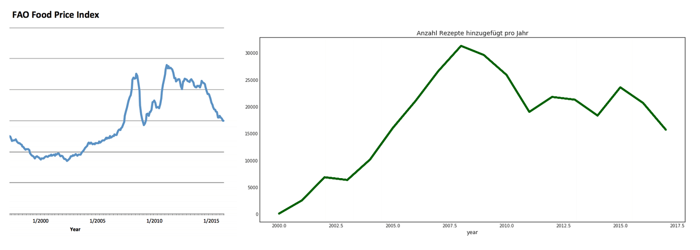
Comparing the curves shows a spurious correlation between the world's rising prices and the supply of recipes. My hypothesis is that demand rose for recipes because people stayed at home and cooked for themselves and their families to save budget and make ends meet as much as possible.
Ingredients
Altogether 316,755 recipes share 3,248,846 ingredients. Removing every ingredient that occurs more than once leaves 63,588 unique ingredients. For the association analysis of the ingredients the APRIORI algorithm is used: it provides how frequently each ingredient occurs in combination with other ingredients.
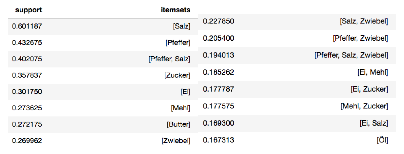
The leader among the ingredients is salt, present in 60 percent of all recipes. In third place comes the first tuple — the combination of two ingredients, pepper and salt — which, at just over 40 percent, is by far the most common pair. The most common triplets, quadruplets and even quintuplets can be found in the corresponding Jupyter notebook, and more graphics in this notebook.
Topic modeling
The data arrived without labels, and a supervised model is not much use without labels, so the categories have to come from the recipes themselves.
The goal of this procedure is to divide all recipe names into n categories. For a supervised classification problem we have to provide the neural network with labelled images; learning is only possible with those labels. The problem is that chefkoch.de does not categorize its pictures. The procedures below split the 316,755 recipe names into categories.
Consider the following example, where four recipe names are given:
- Pizza with mushrooms
- Stuffed peppers with peas and tuna
- Pizza with seafood
- Paprika with peas
These four names must be divided into n categories. Trivially, the first and third recipe belong in the same category, perhaps called pizza. The second and fourth could form another category because of the peas. But how do you correctly categorize more than 300,000 recipe names?
Latent Dirichlet Allocation (LDA)
Probabilistic topic modeling (LDA, Blei et al., 2003) and vector-space models (LSA, Deerwester et al., 1990) approximate the meaning of a word either by modeling documents as finite mixtures over an underlying set of latent topics, or through Singular Value Decomposition (SVD). Since the seminal work of Blei et al. (2003), similar methods (Jagarlamudi et al., 2012) have been proposed to guide the model toward desired topics by providing seed words for each topic, so that the topics are known ahead of time.
As in most NLP tasks, the name body must first be cleaned: stop-words are removed and words are reduced to their root. The clean vocabulary serves as input.
de_stop = get_stop_words('german')
s_stemmer = SnowballStemmer('german')
tokenizer = RegexpTokenizer(r'\w+')

final_names = []
for recipe_name in twentyeigth_iter:
    raw = recipe_name.lower()
    tokens = tokenizer.tokenize(raw)
    stop_t = [recipe_name for recipe_name in tokens
              if not recipe_name in de_stop
              and not recipe_name in filter_words_]
    stem_t = [i for i in stop_t if len(i) > 1]
    if len(stem_t) == 0:
        final_names.append(['error'])
    else:
        final_names.append(stem_t)

print('20 Cleaned Recipe names example: \n >>>')
pprint(final_names[:20])
20 Cleaned Recipe names example:
>>>
[['bratapfel', 'rotkohl'],
['frühstückswolke'],
['deichgrafensalat'],
['geschichteter', 'kohl'],
['rinderlendenragout'],
['blaukraut'],
['sauerbraten'],
['punschtorte'],
['oberländer'],
['mcmoes', 'pasta'],
['geschnetzeltes'],
['ahorn', 'bacon', 'butter'],
['endiviensalat'],
['rote', 'linsen', 'gemüse'],
['kotelett', 'gratin'],
['rotkohl'],
['remouladensauce'],
['nudeln'],
['kohlsuppe'],
['gemüse', 'hackfleischauflauf']]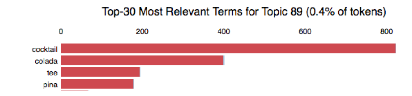
For the sake of simplicity the exact mathematical definition is not discussed here. The result is a list of probabilities expressing how certain the model is that a word fits the topic — for example: 0.363 * "scalloped" + 0.165 * "spicy" + 0.124 * "summer" + 0.006 * "taboulé" + 0.004 * "oatmeal biscuits". An interactive graph for browsing each of the 300 topics is in 04_01_topic_modeling.ipynb in the GitHub repo.
Non-negative Matrix Factorization
The first step is to calculate the TF–IDF (term frequency–inverse document frequency), which represents nothing more than the importance of a word in a recipe name considering its importance across the whole text corpus. The four most important words are:
- salad (2935.18)
- spaghetti (2429.36)
- torte (2196.21)
- cake (1970.08)
The NMF algorithm takes the TF–IDF as input and simultaneously performs dimension reduction and clustering. This yields excellent results, as shown below for the first four topics:
| Topic | Top words |
|---|---|
| #0 | spaghetti carbonara alla olio aglio al sabo puttanesca di mare |
| #1 | salad mixed corn melons chicoree bulgur radish celery quinoa lukewarm |
| #2 | noodles chinese asia mie asian wok udon basil black light |
| #3 | muffins blueberry hazelnut cranberry savory juicy sprinkles johannisbeer oatmeal chocolate |
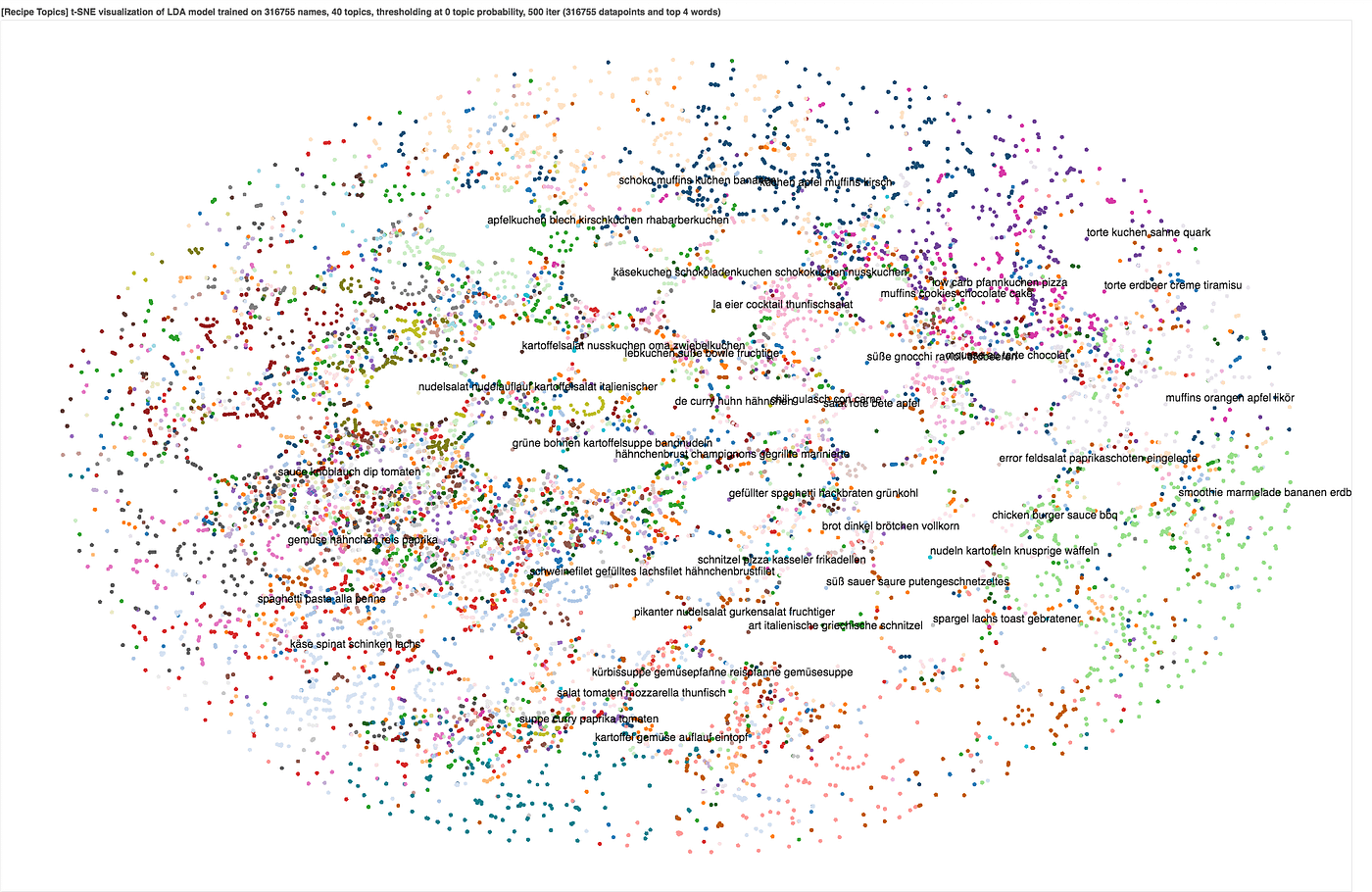
Because we are not crazy people, we start indexing at 0. The result can be visualized with t-SNE: a record with many dimensions is reduced to 2D, which assigns each recipe name a coordinate.
Feature extraction
Names are only half of a recipe. The other half is what the food actually looked like, which is where the pictures finally earn their place.
With CNNs, the image information is first summarized to reduce the number of parameters. We assume that the first layers in a CNN recognize rough structures in the picture, and that the closer you get to the last Softmax layer, the finer the learned features become. We can take advantage of this: we take pre-trained CNNs that have been trained on millions of pictures and remove the last layers so as to retrain them with our own data. This saves us millions of parameters and so reduces computing time. The CNN chosen here is VGG-16, trained in the 2014 classification competition on 1,000 categories.
If you remove the last layer you get a feature extractor at the second-to-last layer. This forms an n × 4096 matrix, where n is the number of input pictures.
features = []
for image_path in tqdm(images):
    img, x = get_image(image_path);
    feat = feat_extractor.predict(x)[0]
    features.append(feat)
We let VGG-16 calculate the vector for every image we have. This vector is, so to speak, the fingerprint of the picture: an internal representation the neural network builds.
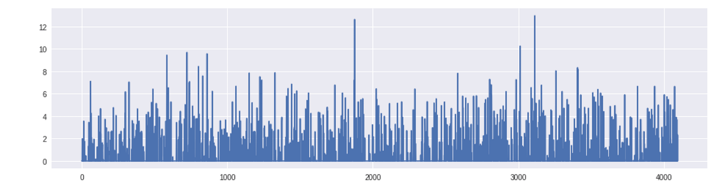
Now, for every new input image, all we have to do is pass it through VGG-16, get the fingerprint vector and calculate the nearest neighbours with approximate nearest-neighbour search. The library used here is FALCONN, a library of algorithms for the nearest-neighbour search problem. The algorithms in FALCONN are based on Locality-Sensitive Hashing (LSH), a popular class of methods for nearest-neighbour search in high-dimensional spaces. The goal of FALCONN is to provide very efficient and well-tested implementations of LSH-based data structures.
FALCONN currently supports two LSH families for the cosine similarity: hyperplane LSH and cross-polytope LSH. Both are implemented with multi-probe LSH to minimize memory usage, and FALCONN is optimized for both dense and sparse data. Despite being designed for cosine similarity, FALCONN can often be used for nearest-neighbour search under the Euclidean distance, or for a maximum inner-product search.
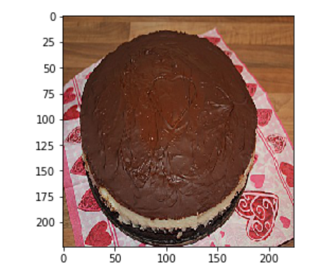
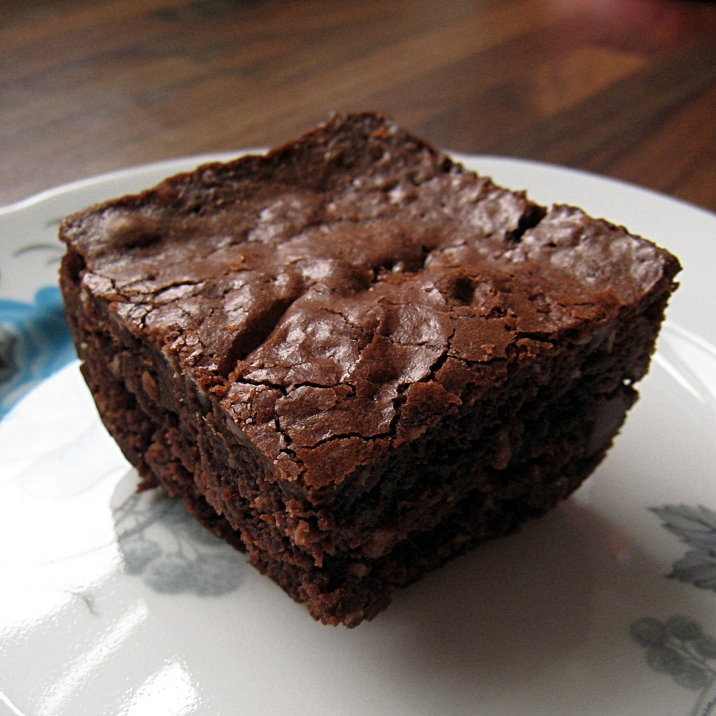
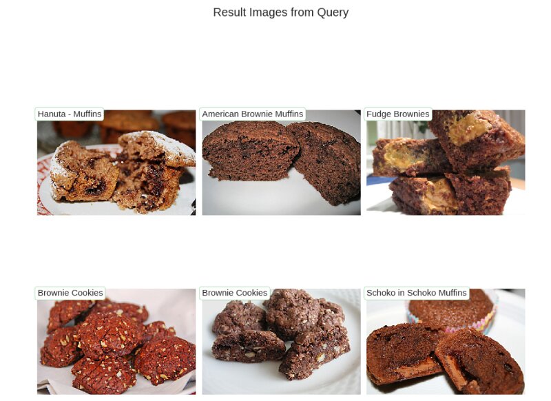
To test the chosen ANN approach, we pass the brownie image on the left (Figure 9) and, as expected, receive similarly looking dishes.
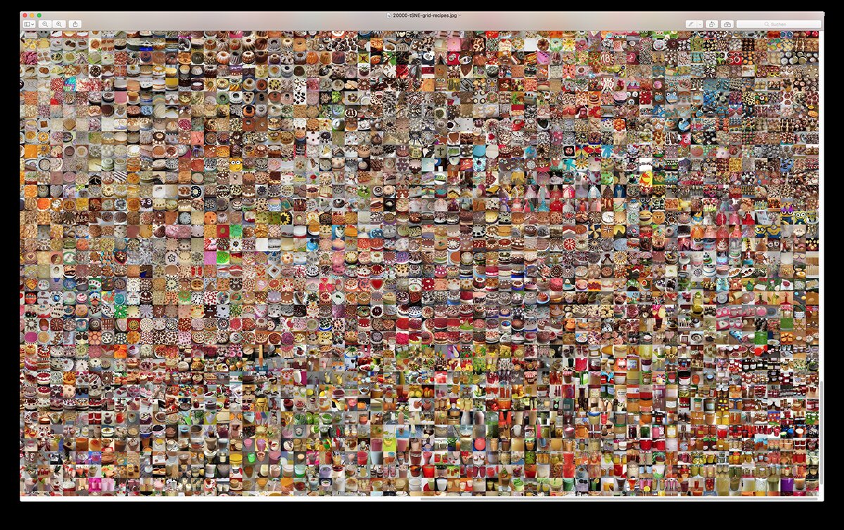
We can even create a grid of images to view the neural network's interpretation. The picture below is only a small part of the whole image; cooking dishes that share similar features sit closer together. The whole grid can be found here.
Conclusion
We have introduced a new dataset that jointly represents cooking images with their corresponding recipes. We have highlighted the important differences between the chosen food domain and pre-existing image-classification tasks, and empirically investigated the effectiveness of convolutional neural networks and approximate nearest-neighbour methods.
How to train your own neural network from scratch without pre-training, and how to turn the system into a web application with Flask (Part V and Part VI), will be covered in the next tutorial. Find out more at muriz.ch, and browse the full code in the GitHub repository.
Cite this article
If this was of any use, the kindest citation is telling someone about it; the entry below covers the less kind occasions.
@article{serifovic2018recipecnn,
  author  = {Serifovic, Muriz},
  title   = {Image-to-Recipe Translation with Deep Convolutional Neural Networks},
  journal = {muriz.ch},
  year    = {2018},
  month   = {September},
  note    = {https://muriz.ch/blog/image-to-recipe-translation.html},
}