Persistent Homology and the Topology of Neurodegenerative Disease

Introduction

Many neurodegenerative diseases share a common pathological signature: misfolded proteins accumulating in the nervous system. ⊕Jucker, M., & Walker, L. C. (2018). Propagation and spread of pathogenic protein assemblies in neurodegenerative diseases. Nature Neuroscience, 21(10), 1341–1349. In Alzheimer's disease (AD), amyloid-$\beta$ plaques and tau tangles progressively disrupt neural circuits. In Parkinson's disease, $\alpha$-synuclein aggregates spread through connected brain regions. These proteins follow existing neural pathways as they spread.

Neuroimaging studies show that neurodegeneration patterns match the brain's structural and functional connectome surprisingly well. ⊕Garbarino, S., et al. (2019). Differences in topological progression profile among neurodegenerative diseases from imaging data. eLife, 8, e49298. So understanding the topology of brain networks, their global shape and connectivity structure, might tell us something about how disease spreads.

This article introduces persistent homology, a technique from algebraic topology for capturing multi-scale topological features in networks. I'll develop the mathematical machinery (simplicial complexes, chain groups, boundary operators, homology), then show how these tools apply to brain network analysis in Alzheimer's research, following Kuang et al. (2020). ⊕Kuang, L., et al. (2020). White matter brain network research in Alzheimer's disease using persistent features. Molecules, 25(11), 2472.

From brain networks to topology

The human brain can be modeled as a weighted graph $G = (V, E, w)$, where vertices $V$ are brain regions (typically defined by an anatomical atlas), edges $E$ are structural or functional connections, and weights $w: E \to \mathbb{R}$ quantify connection strength. From diffusion tensor imaging (DTI), you can construct a structural connectivity matrix encoding white matter fiber density between regions.

Classical graph-theoretic measures (characteristic path length, clustering coefficient, modularity) have been useful for characterizing brain networks. But these measures depend on choosing a threshold: edges below a certain weight get discarded, and the analysis proceeds on the resulting binary graph. Different thresholds yield different networks. There's no principled way to select the "correct" one.

Persistent homology offers an alternative. Instead of fixing a single threshold, we consider all thresholds simultaneously. As we vary the threshold from strict to permissive, topological features (connected components, loops, voids) appear and disappear. Features that persist across a wide range of thresholds are considered "real" structure; those that appear briefly are likely noise. This multi-scale perspective is what topological data analysis is about.

To make this precise, we need the language of algebraic topology: simplicial complexes to represent our data, chain complexes to encode combinatorial structure, and homology to measure topological features.

Mathematical preliminaries

Simplicial complexes

The building blocks here are simplices, the higher-dimensional generalizations of points, line segments, triangles, and tetrahedra.

Definition. A $k$-simplex $\sigma = [v_0, v_1, \ldots, v_k]$ is the convex hull of $k+1$ affinely independent points in some Euclidean space: $$ \sigma = \left\{ \sum_{i=0}^{k} \lambda_i v_i \;\middle|\; \lambda_i \geq 0,\; \sum_{i=0}^{k} \lambda_i = 1 \right\}. $$ A $0$-simplex is a vertex, a $1$-simplex is an edge, a $2$-simplex is a (filled) triangle, and a $3$-simplex is a (solid) tetrahedron. 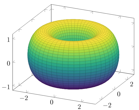⊕A torus has Betti numbers $\beta_0=1$, $\beta_1=2$, $\beta_2=1$: one connected component, two independent loops, and one void.

Definition. A face of a simplex $\sigma = [v_0, \ldots, v_k]$ is any simplex spanned by a non-empty subset of its vertices. We write $\tau \leq \sigma$ if $\tau$ is a face of $\sigma$, and $\tau < \sigma$ if $\tau$ is a proper face (i.e., $\tau \neq \sigma$).

Definition. A simplicial complex $K$ is a finite collection of simplices satisfying two conditions:

1. If $\sigma \in K$ and $\tau \leq \sigma$, then $\tau \in K$ (closure under taking faces).
2. If $\sigma, \tau \in K$, then $\sigma \cap \tau$ is either empty or a face of both $\sigma$ and $\tau$.

Chain groups and the boundary operator

To extract algebraic information from a simplicial complex, we need chain groups and the boundary operator. I follow Hatcher's notation throughout. ⊕Hatcher, A. (2002). Algebraic Topology. Cambridge University Press. Freely available at pi.math.cornell.edu/~hatcher.

Definition. The $k$-th chain group $C_k(K)$ of a simplicial complex $K$ is the free abelian group generated by the $k$-simplices of $K$. An element of $C_k(K)$ is a $k$-chain: a formal linear combination $$ c = \sum_i a_i \sigma_i, \quad a_i \in \mathbb{Z}, $$ where $\sigma_i$ ranges over the $k$-simplices of $K$.

Definition. The boundary operator $\partial_k: C_k(K) \to C_{k-1}(K)$ is the homomorphism defined on generators by $$ \partial_k [v_0, v_1, \ldots, v_k] = \sum_{i=0}^{k} (-1)^i [v_0, \ldots, \widehat{v_i}, \ldots, v_k], $$ where $\widehat{v_i}$ indicates that vertex $v_i$ is omitted. The alternating signs encode orientation.

Example. For a $2$-simplex (triangle) $[v_0, v_1, v_2]$: $$ \partial_2 [v_0, v_1, v_2] = [v_1, v_2] - [v_0, v_2] + [v_0, v_1]. $$ The boundary of a triangle is the sum of its three edges, with signs reflecting consistent orientation around the triangle.

The chain groups and boundary operators assemble into a chain complex:

The key property: the composition of two consecutive boundary operators is zero: $$ \partial_{k-1} \circ \partial_k = 0 \quad \text{for all } k. $$ Or as topologists like to say: "the boundary of a boundary is empty." This algebraic identity reflects a geometric fact. A filled triangle has an edge boundary, but that boundary (a closed loop of edges) has no boundary of its own.

Homology groups

The property $\partial \circ \partial = 0$ implies that $\operatorname{im}(\partial_{k+1}) \subseteq \ker(\partial_k)$. This inclusion is what makes homology possible.

Definition. The $k$-cycles are chains with zero boundary: $$ Z_k(K) = \ker(\partial_k) = \{ c \in C_k(K) \mid \partial_k c = 0 \}. $$ The $k$-boundaries are chains that are boundaries of $(k+1)$-chains: $$ B_k(K) = \operatorname{im}(\partial_{k+1}) = \{ \partial_{k+1} c \mid c \in C_{k+1}(K) \}. $$

Definition. The $k$-th homology group of $K$ is the quotient $$ H_k(K) = Z_k(K) / B_k(K). $$ Elements of $H_k(K)$ are equivalence classes of cycles: two cycles are homologous if their difference is a boundary.

Definition. The $k$-th Betti number is $\beta_k(K) = \operatorname{rank}(H_k(K))$.

Interpretation. Betti numbers count topological features:

• $\beta_0$: number of connected components
• $\beta_1$: number of independent loops (or "tunnels")
• $\beta_2$: number of enclosed voids (or "cavities")

Functoriality of homology

Homology is functorial: continuous maps between spaces induce homomorphisms between their homology groups.

Proposition. If $f: K \to L$ is a simplicial map (sending simplices to simplices, preserving face relations), then $f$ induces a chain map $f_\#: C_k(K) \to C_k(L)$ that commutes with the boundary operators. This, in turn, induces a homomorphism on homology: $$ f_*: H_k(K) \longrightarrow H_k(L). $$

In particular, if $K \subseteq L$ is a subcomplex, the inclusion $\iota: K \hookrightarrow L$ induces maps $\iota_*: H_k(K) \to H_k(L)$. This is what makes persistent homology work: as we build up a complex through a filtration, we can track how homology classes evolve.

Persistent homology

Filtrations

Definition. A filtration of a simplicial complex $K$ is a nested sequence of subcomplexes $$ \emptyset = K_0 \subseteq K_1 \subseteq K_2 \subseteq \cdots \subseteq K_n = K, $$ where each inclusion $K_i \hookrightarrow K_{i+1}$ adds one or more simplices.

Filtrations arise naturally from data. Given a weighted graph $G = (V, E, w)$, we can define a graph filtration by including edges in order of increasing weight: at threshold $\epsilon$, we include all edges with $w(e) \leq \epsilon$. As $\epsilon$ increases, more edges appear, and the topology of the resulting complex evolves.

Each inclusion $\iota_i: K_i \hookrightarrow K_{i+1}$ induces a homomorphism on homology $(\iota_i)_*: H_k(K_i) \to H_k(K_{i+1})$. The collection of all these homology groups and induced maps forms a persistence module:

Birth, death, and persistence

As we traverse a filtration, homology classes appear and disappear. A homology class $\alpha \in H_k(K_i)$ is born at index $i$ if it's not in the image of the map $H_k(K_{i-1}) \to H_k(K_i)$. In other words, $\alpha$ is a genuinely new topological feature that didn't exist at the previous stage.

A class born at $i$ dies at index $j > i$ if its image in $H_k(K_j)$ becomes trivial (the class becomes a boundary). The persistence of such a class is $j - i$: how long the feature survives across the filtration.

Definition. The $(i,j)$-persistent $k$-th Betti number is $$ \beta_k^{i,j} = \operatorname{rank}\bigl(\operatorname{im}(H_k(K_i) \to H_k(K_j))\bigr), $$ counting how many $k$-dimensional features born at or before $i$ survive until at least $j$.

Persistence diagrams and barcodes

The birth-death pairs $(b, d)$ of all homology classes can be visualized two ways:

Persistence diagram. A multiset of points in the plane, where each point $(b, d)$ is a feature born at filtration value $b$ and dying at $d$. Points far from the diagonal $b = d$ are long-lived features; points near the diagonal are noise.

Barcode. A collection of horizontal intervals $[b, d)$, one per feature. Long bars are persistent features; short bars are ephemeral ones.

In this schematic barcode, we see four connected components ($\beta_0$ features) appearing at different times, three of which eventually merge (die) while one persists to the end. Two loops ($\beta_1$ features) appear later in the filtration; one persists longer than the other.

The Vietoris-Rips construction

Given a finite metric space $(X, d)$, say a set of brain regions with pairwise distances, we can build a simplicial complex whose topology reflects the geometry of $X$.

Definition. The Vietoris-Rips complex at scale $\epsilon \geq 0$ is $$ \operatorname{VR}_\epsilon(X) = \bigl\{ \sigma \subseteq X \;\big|\; \operatorname{diam}(\sigma) \leq \epsilon \bigr\}, $$ where $\operatorname{diam}(\sigma) = \max_{x,y \in \sigma} d(x,y)$. In other words, a subset $\sigma \subseteq X$ forms a simplex if and only if every pair of points in $\sigma$ is within distance $\epsilon$.

As $\epsilon$ increases, more simplices appear, yielding a filtration $\operatorname{VR}_0(X) \subseteq \operatorname{VR}_{\epsilon_1}(X) \subseteq \cdots$. Applying persistent homology to this filtration reveals the multi-scale topological structure of $X$.

Application to brain networks in Alzheimer's disease

Kuang et al. (2020) applied persistent homology to structural brain networks from diffusion tensor imaging (DTI) in 150 subjects: 50 with Alzheimer's disease (AD), 50 with mild cognitive impairment (MCI), and 50 normal controls (NC). They parcellated the brain into 68 regions using the Desikan-Killiany atlas, with edge weights computed from white matter fiber connectivity: $$ w_{ij} = 1 - \operatorname{corr}(T_i, T_j), $$ where $T_i$ and $T_j$ are fiber connection profiles. Lower weights mean stronger connectivity.

Instead of constructing Vietoris-Rips complexes directly, they used a graph filtration based on the minimum spanning tree (MST). Varying the threshold $\lambda$ from 0 to 1.3, they tracked the zeroth Betti number $\beta_0(\lambda)$ (the number of connected components) across the filtration. What they found:

⊕From Kuang et al. (2020), Figure 2: "Multiscale WM networks of the three groups, AD (a), MCI (b), and NC (c), at some filtrations. The AD group shows more sparse connections (more segregated components) compared to controls when $\lambda \leq 0.8$."

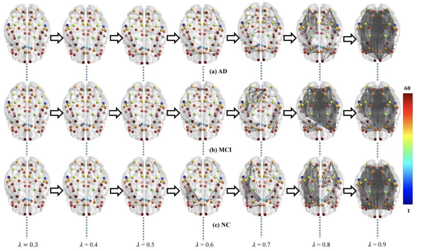
• AD brains showed more fragmented networks (higher $\beta_0$) at low filtration values, indicating disrupted connectivity.
• Persistent features, specifically the Betti number plot (BNP) and integrated persistent feature (IPF), distinguished AD, MCI, and NC with statistical significance ($p < 0.01$).
• These topological markers were more robust than classical graph metrics across different brain parcellation schemes.

Discussion

Applying persistent homology to brain networks is a shift from local to global analysis. Classical graph metrics (clustering coefficients, path lengths, centrality measures) capture local structure but are sensitive to thresholding choices. Persistent homology sidesteps this by considering all thresholds simultaneously and extracting features that persist across scales.

The mathematics here (simplicial complexes, chain complexes, homology, persistence) gives us a foundation for multi-scale network analysis. The point is functoriality: inclusions of complexes induce maps on homology, so we can track topological features as the network evolves.

Some directions I find interesting: higher-dimensional persistent homology ($\beta_1$, $\beta_2$) might capture subtler network structure. Stability theorems guarantee that small perturbations in input data yield small changes in persistence diagrams, which helps with measurement noise. And the algebraic structure of persistence modules, particularly their decomposition into interval summands, hasn't been fully exploited in neuroimaging yet.